이진 분류
Output층에 활성화 함수는 Sigmoid함수를 사용한다.
0 ~ 1 사이 확률 값으로 변환해주는 역할을 한다.
Loss Function으로는 binary_crossentropy를 사용한다.
오차들의 평균 계산
1. output 층에 활성화함수는 시그모이드가 필요
# 메모리 정리
clear_session()

# Sequential 모델 만들기
model = Sequential( [Input(shape = (nfeatures,)),
                    Dense(50, activation='relu'),
                    Dense(1, activation='sigmoid')])
# 모델요약
model.summary()
2. 손실 함수는 binary_crossentropy
model.compile(optimizer = Adam(learning_rate=0.01), loss = 'binary_crossentropy')

history = model.fit(x_train, y_train, epochs = 50, validation_split=0.2).history
3. 0.5를 기준으로 나누기
pred = model3.predict(x_val)
pred = np.where(pred >= 0.5, 1, 0)
4. 검증
print(classification_report(y_val, pred))
다중 분류
필요한 y만큼 output 수를 맞추어야 한다.
하지만 output에서 나온 각 숫자들를 실제값인 확률값으로 변환시켜야 한다.
이를 활성화 함수 softmax가 바꾸어 준다.
방법 ① : 정수 인코딩 + sparse_categorical_crossentropy
- 정수 인코딩(0,1,2 등)
data['Species'] = data['Species'].map({'setosa':0, 'versicolor':1, 'virginica':2})
※ 주의 - 항상 0 부터 시작해야 함
# 데이터 준비
target = 'Species'
x = data.drop(target, axis = 1)
y = data.loc[:, target]

# 데이터 분할
x_train, x_val, y_train, y_val = train_test_split(x, y, test_size = .3, random_state = 20)

# 스케일링
scaler = MinMaxScaler()
x_train = scaler.fit_transform(x_train)
x_val = scaler.transform(x_val)
- 활성화 함수 : softmax
# 메모리 정리
clear_session()

# Sequential
model = Sequential( [Input(shape = (nfeatures,)),
                     Dense( 3, activation = 'softmax')] )

# 모델요약
model.summary()
- 손실 함수 : sparse_categorical_crossentropy
model.compile(optimizer=Adam(learning_rate=0.1), loss= 'sparse_categorical_crossentropy')

history = model.fit(x_train, y_train, epochs = 50, validation_split=0.2).history
#dl_history_plot(history)
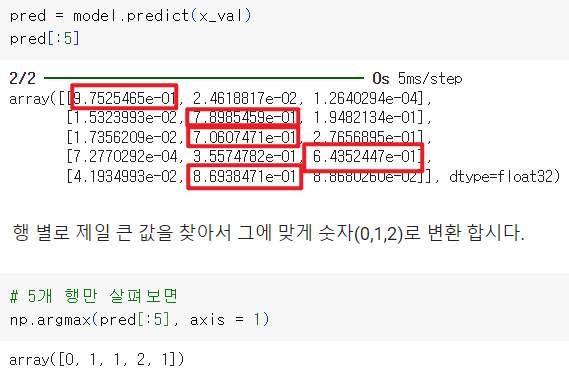
- 모델 평가 : 큰 값의 인덱스 찾기
pred = model.predict(x_val)
pred_1 = pred.argmax(axis=1)
print(confusion_matrix(y_val, pred_1))
print(classification_report(y_val, pred_1))
방법 ② : 원핫 인코딩 + categorical_crossentropy
- 정수 인코딩 필요
data['Species'] = data['Species'].map({'setosa':0, 'versicolor':1, 'virginica':2})
- 원핫 인코딩
from keras.utils import to_categorical
y_c = to_categorical(y.values, 3)
x_train, x_val, y_train, y_val = train_test_split(x, y_c, test_size = .3, random_state = 2022)
scaler = MinMaxScaler()
x_train = scaler.fit_transform(x_train)
x_val = scaler.transform(x_val)
# 메모리 정리
clear_session()

# Sequential
model = Sequential([Input(shape = (nfeatures,)),
                    Dense(3, activation = 'softmax')])

# 모델요약
model.summary()
- 손실 함수 : categorical_cossentopy
model.compile(optimizer=Adam(learning_rate=0.1), loss='categorical_crossentropy')

history = model.fit(x_train, y_train, epochs = 100,
                    validation_split=0.2).history
- 평가
실제값 y_val도 원래 값으로 변경
pred = model.predict(x_val)
pred_1 = pred.argmax(axis=1)
y_val_1 = y_val.argmax(axis=1)
print(confusion_matrix(y_val_1, pred_1))
print(classification_report(y_val_1, pred_1))
- 학습 곡선 함수
더보기
# 학습곡선 함수
def dl_history_plot(history):
    plt.figure(figsize=(10,6))
    plt.plot(history['loss'], label='train_err', marker = '.')
    plt.plot(history['val_loss'], label='val_err', marker = '.')

    plt.ylabel('Loss')
    plt.xlabel('Epoch')
    plt.legend()
    plt.grid()
plt.show()'KT AIVLE School > 딥러닝' 카테고리의 다른 글
| 시계열 모델링 (0) | 2024.10.15 |
|---|---|
| Functional API 및 다중 입력 (0) | 2024.10.15 |
| 모델 저장하기 (0) | 2024.10.14 |
| 적절한 복잡도 찾기 (2) | 2024.10.14 |
| 회귀모델링 (1) | 2024.10.11 |